Thermal Modeling with State Space

Introduction: The Need for Multi-Fidelity Thermal Modeling

With the rise of 2.5D and 3D integration in chiplet-based systems, thermal management has become a critical challenge. The compact designs lead to higher thermal densities, and conventional methods either lack the speed or accuracy to evaluate temperature reliably across such systems. Our proposed framework, MFIT, addresses this gap by introducing multi-fidelity thermal models that balance accuracy and execution speed. This suite of models enables designers to explore trade-offs at different phases of chip design and thermal-aware optimization.

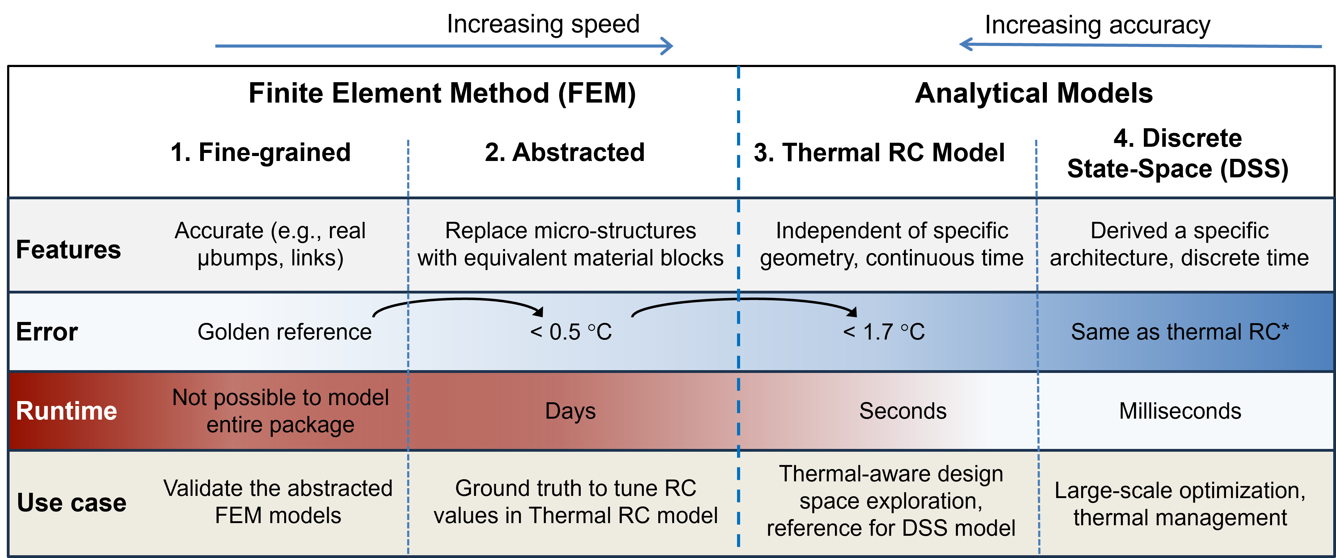
MFIT provides models ranging from finite element method (FEM) for high-accuracy thermal analysis to thermal RC and discrete-state space (DSS) models for faster approximations. Together, these models enable designers to simulate and manage thermal dynamics efficiently, from design exploration to real-time thermal management.

Finite Element Method (FEM) Analysis

FEM Basics: Solving PDEs for Heat Transfer

The FEM is the most accurate method for thermal analysis, solving the heat conduction equation:

Here, \(k\) is thermal conductivity, \(T\) is temperature, \(\dot{q}\) is heat generation rate, \(\rho\) is density, and \(c\) is volumetric specific heat.

FEM begins by creating the system geometry into a mesh of finite elements. The partial differential equations (PDEs) governing heat transfer are applied to each element, and boundary conditions are incorporated. We used industry-standard tools ANSYS Fluent for solving these equations, providing precise temperature distributions across complex geometries.

FEM Challenges

Despite its accuracy, FEM simulations are computationally expensive and time-consuming, especially for large multi-chiplet systems. This limitation makes FEM impractical for real-time or large-scale design space exploration, motivating the need for abstraction.

From FEM to Thermal RC: Discretization in Space

The Thermal RC Model

The thermal RC model approximates the FEM solution by discretizing the geometry into thermal resistances and capacitances, analogous to an electrical RC network. This process transforms the continuous PDEs into a system of ordinary differential equations (ODEs), which can be solved using advanced solvers such as LSODA.

The Thermal RC Model Formulation

To efficiently approximate heat transfer, we replace the FEM-based spatially continuous model with a thermal RC network, where the thermal conductance and capacitance are calculated for each node.

Continuous-Time ODE Formulation

Based on Kirchhoff’s current law for heat transfer, the temperature dynamics of each node are modeled using the following ordinary differential equation (ODE):

where:

• \(C_i\): Thermal capacitance of node \(i\),
• \(G_{ij}\): Thermal conductance between node \(i\) and its neighbor \(j\),
• \(T_i\) and \(T_j\): Temperatures of nodes \(i\) and \(j\),
• \(\dot{q}_i\): Heat generation at node \(i\).

Matrix Representation

To solve the system of ODEs efficiently, we represent it in matrix form (please refer to our paper for detailed derivations):

where:

• for \(N\) nodes, \(\mathbf{C}\) is an \(N\) dimensional diagonal matrix of thermal capacitances,
• \(\mathbf{G}\) is the conductance matrix of size \(N \times N\),
• \(\mathbf{T}\) is the temperature vector of size \(N\), and
• \(\dot{\mathbf{q}}\) is the heat generation rate vector of size \(N\).

Key Features of the Thermal RC Model

1. Directional Conductivity: Unlike previous models, MFIT supports varying thermal conductivities in \(x\), \(y\), and \(z\)-directions, enabling more accurate modeling of materials like interposers and chiplets.
2. Non-uniform Grid Resolution: The model allows different numbers of nodes for each block, enhancing the fidelity for thermally critical regions without increasing computational overhead.

Why LSODA?

LSODA dynamically switches between stiff and non-stiff solvers, outperforming other approaches in accuracy and efficiency. Its adaptability is crucial for solving the thermal RC ODEs, becuse the system can exhibit both stable and dynamic power profiles.

From Thermal RC to Discrete State Space (DSS): Discretization in Time

Transitioning to DSS Models

The discrete-state space (DSS) model further simplifies the thermal RC network by discretizing time. This approach assumes power remains constant over small time intervals, similar to how power-monitoring tools like Intel RAPL and NVIDIA pyNVML compute running averages.

The resulting model uses a linear time-invariant system to represent thermal dynamics, making it ideal for real-time applications. DSS models significantly reduce simulation time while retaining sufficient accuracy for dynamic thermal management and design optimization.

DSS Model Formulation

Step 1: Convert to the Standard Continuous-Time Form

Rewriting the given equation:

This is the standard continuous-time state-space form.

Step 2: Solution of the Continuous-Time State Equation

The solution for \(\dot{\mathbf{T}} = \mathbf{A} \mathbf{T} + \mathbf{B} \dot{\mathbf{q}}\) over a time interval \(t \in [kT_s, (k+1)T_s]\) is obtained by integrating the dynamics. (where \(T_s\) is the sampling period and \(k\) is the time index.)

1. Homogeneous Solution (due to \(\mathbf{A} \mathbf{T}\)):
   Assuming no inputs (\(\dot{\mathbf{q}} = 0\)), the state evolves as:

   \[\mathbf{T}(t) = e^{\mathbf{A} (t - kT_s)} \mathbf{T}(kT_s),\]

   where \(e^{\mathbf{A}(t-kT_s)}\) is the matrix exponential.

2. Particular Solution (due to \(\mathbf{B} \dot{\mathbf{q}}\)):
   When \(\dot{\mathbf{q}}\) is present and constant during \(t \in [kT_s, (k+1)T_s]\) (ZOH assumption), the particular solution is:

   \[\mathbf{T}(t) = \int_{kT_s}^{t} e^{\mathbf{A}(t - \tau)} \mathbf{B} \dot{\mathbf{q}}(\tau) \, d\tau.\]

   Substituting \(\dot{\mathbf{q}}(\tau) = \dot{\mathbf{q}}(kT_s)\), this simplifies to:

   \[\int_{kT_s}^{t} e^{\mathbf{A}(t - \tau)} \mathbf{B} \, d\tau \cdot \dot{\mathbf{q}}(kT_s).\]

Adding these, the total solution is:

Step 3: Discretization

At \(t = (k+1)T_s\), the discrete-time model becomes:

if \(\mathbf{A}\) is invertible, the integral can be computed as:

Discrete-time matrices:

Thus, the discrete-time state-space equation is:

Limitations of DSS Models

While DSS models are computationally efficient, their accuracy depends on the availability of a precomputed thermal RC model. This dependency limits their applicability in scenarios lacking detailed geometric or material information.

To explore our codebase and learn more, read our paper MFIT: Multi-Fidelity Thermal Modeling for 2.5D and 3D Multi-Chiplet Architectures and visit the MFIT GitHub Repository.